Thank you to my advisor, committee, friends, family, labmates, and collaborators.
Motivation
Motivation
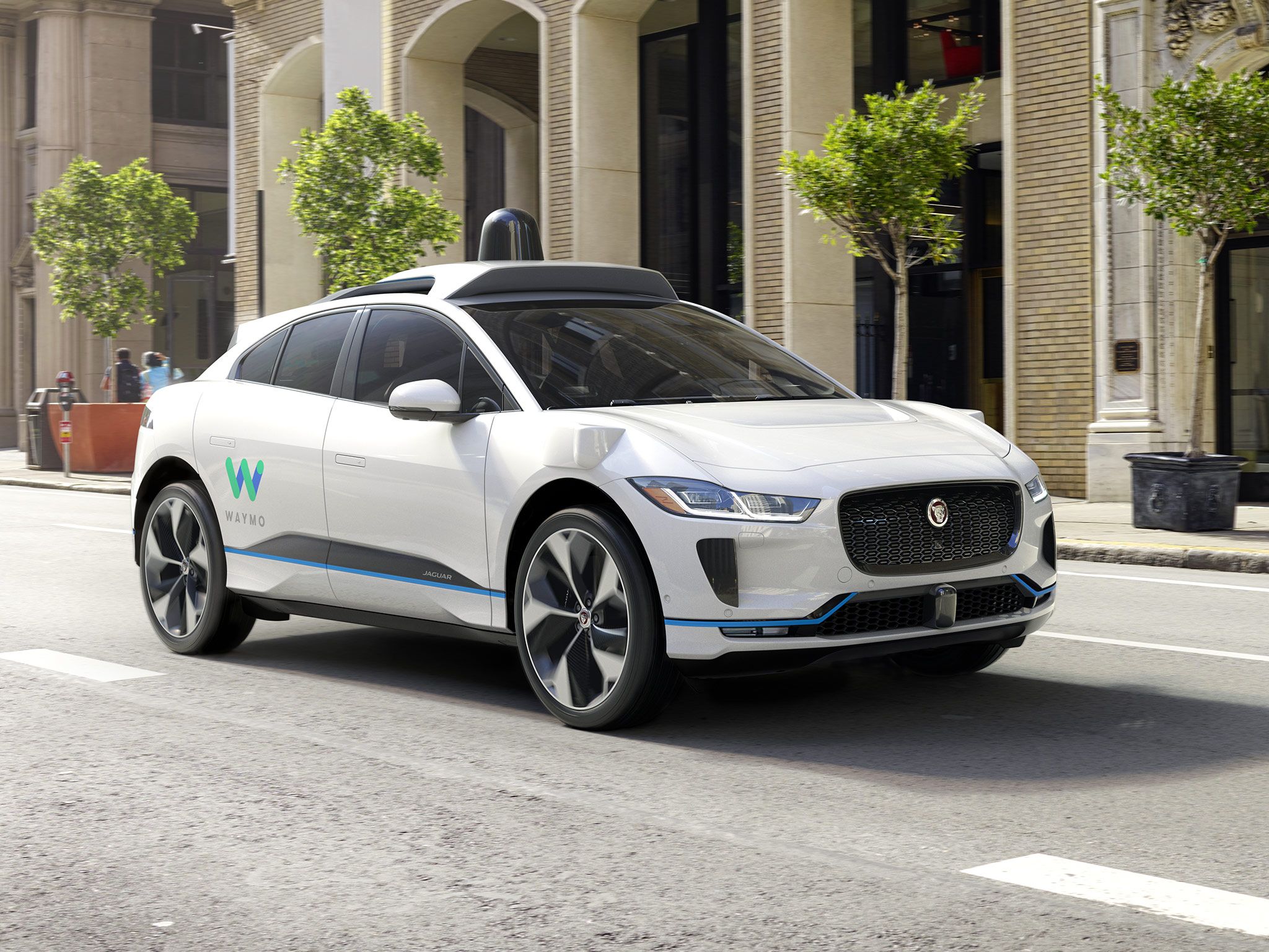
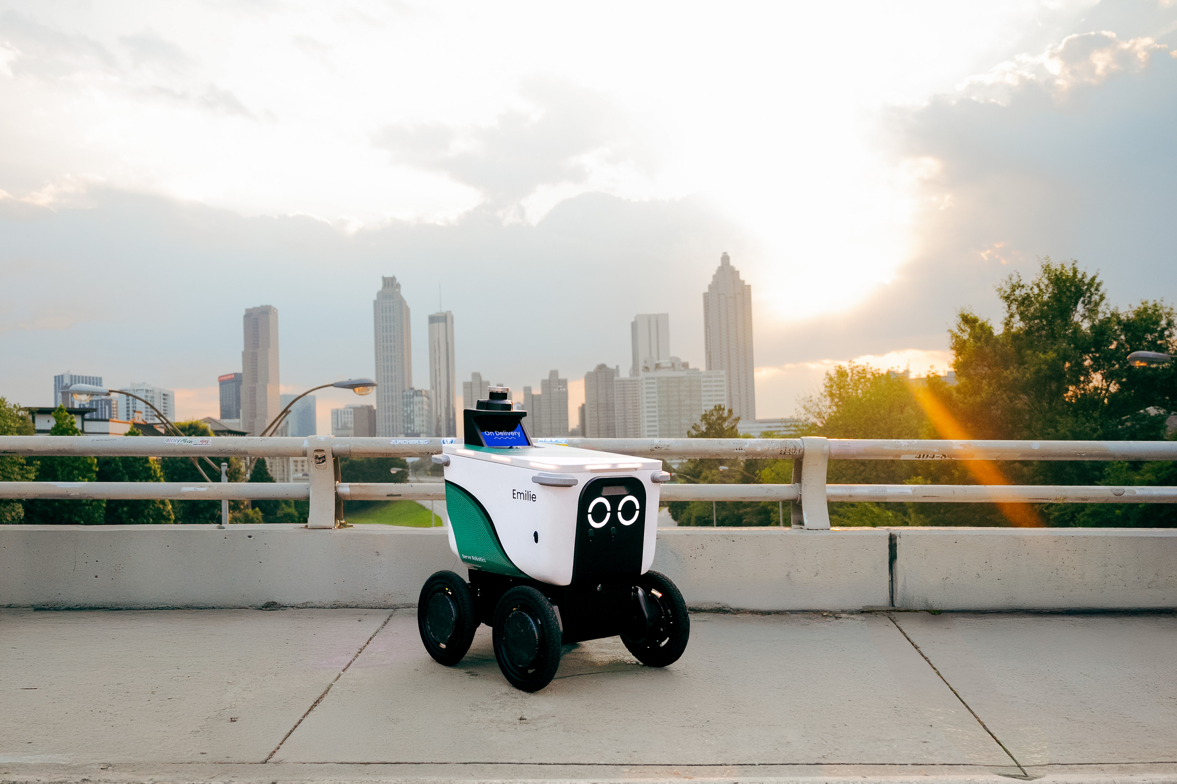
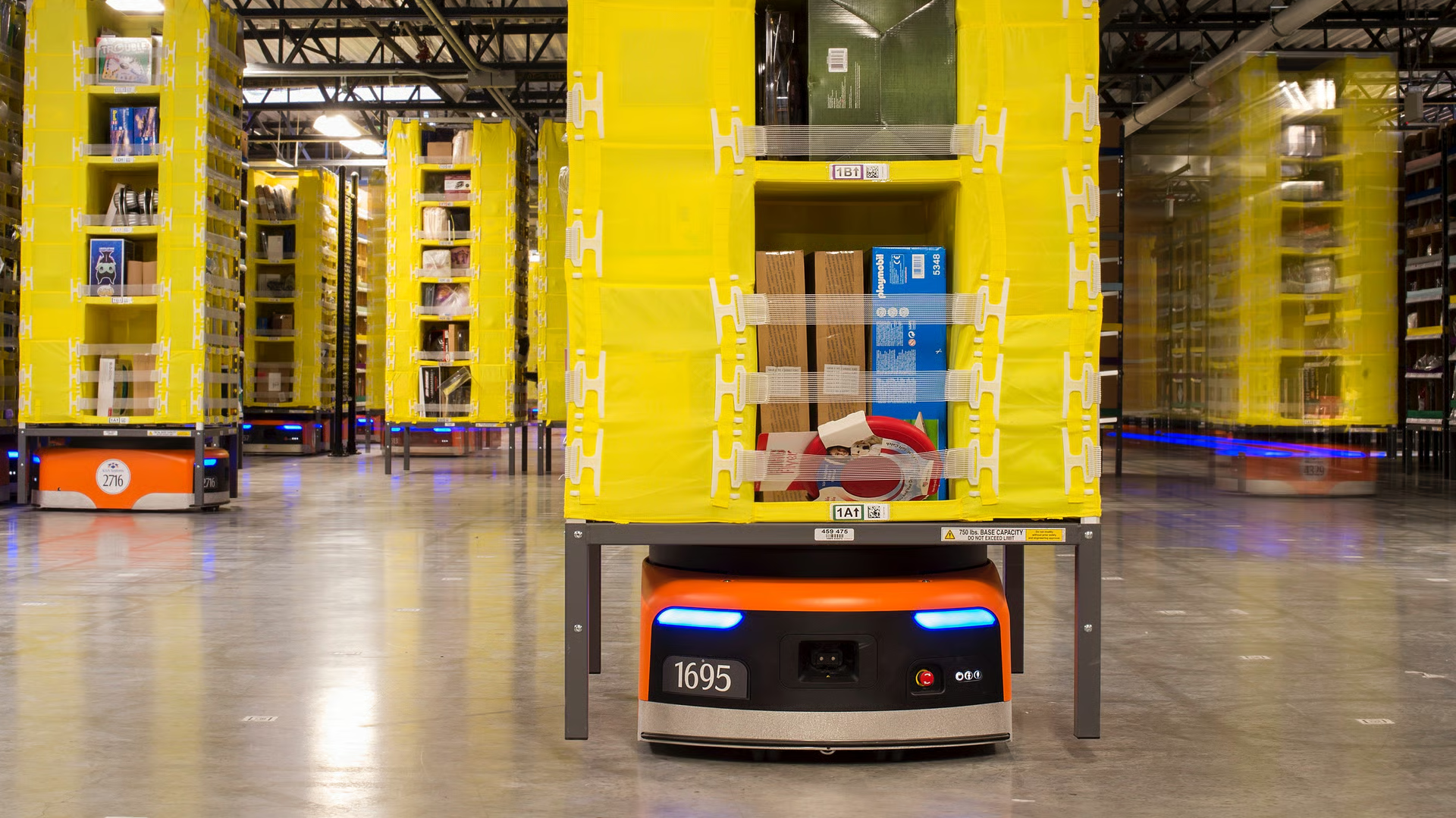
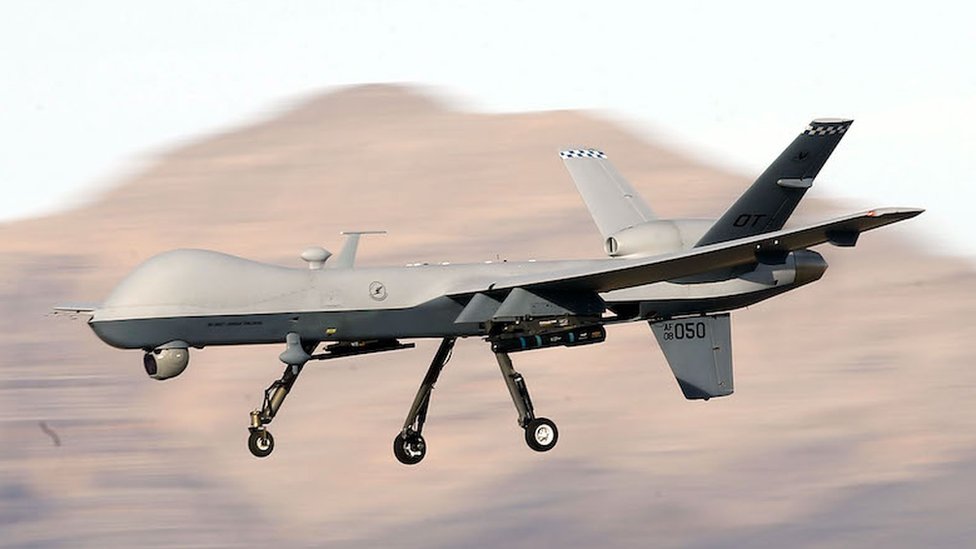
Autonomous robotics are an increasingly prominent part of our lives — on our roads and sidewalks, in our warehouses and supply chains, and in the skies above.
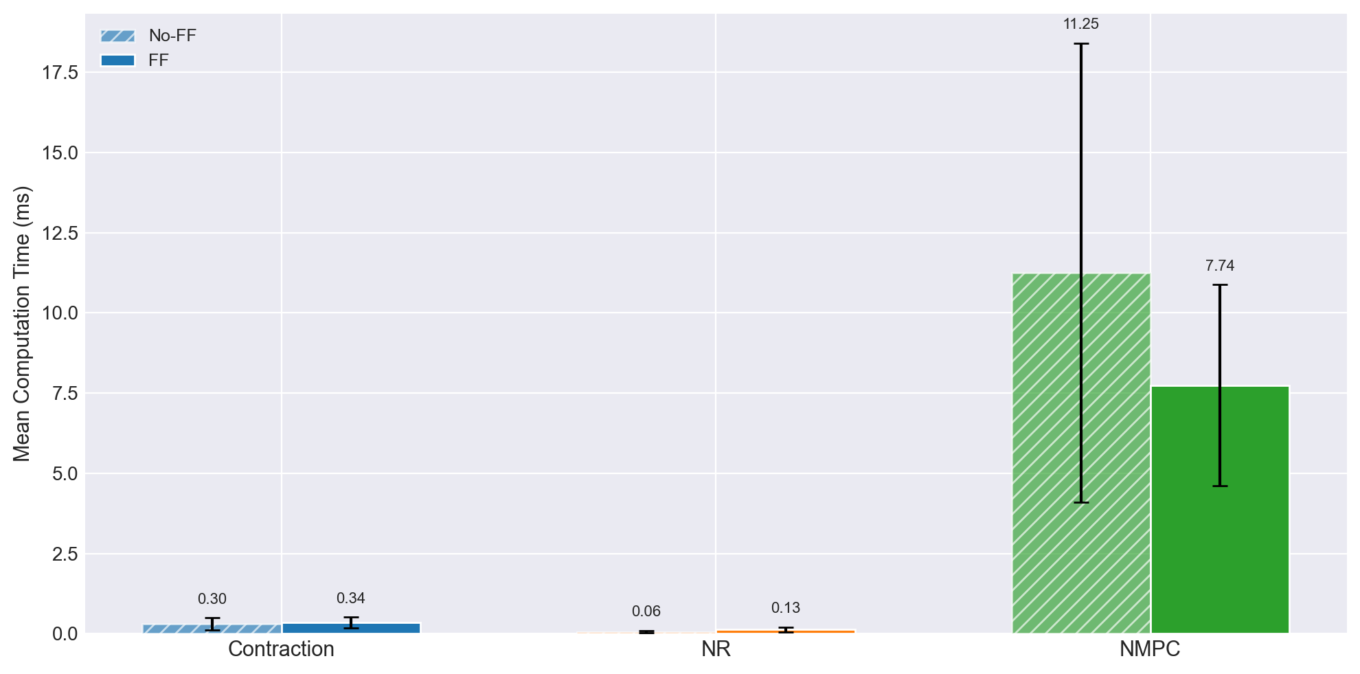
A drone in mid-flight may suddenly deviate from its intended trajectory, leaving only a narrow time window to diagnose the anomaly and apply corrective action before failure becomes unavoidable.
Despite major advances in aerial trajectory planning and control, state-of-the-art methods remain time- and compute-heavy — hard to deploy on real hardware.
Particularly pronounced on miniature aerial platforms, where onboard compute is often limited
NMPC is the state-of-the-art, yet: “impractical to run NMPC on some miniature aerial vehicles with a limited computational budget”[1]
Similar state-of-the-art approaches are either computationally complex, or require advanced reference derivatives or detailed model knowledge
The practical state-of-the-art remains largely tethered to advanced PID control — a gap between the practical and research state-of-the-art.
Newton–Raphson Flow Controller
For \(\dot x = f(x,u),\; y = h(x)\), introduce a differentiable look-ahead predictor \(\hat y(t+T) = \rho(x(t), u(t))\) under zero-order hold on \(u\). Applying NRT to the predictor [2]:
For \(\dot x = f(x,u),\; y = h(x)\), introduce a differentiable look-ahead predictor \(\hat y(t+T) = \rho(x(t), u(t))\) under zero-order hold on \(u\). Applying NRT to the predictor [2]:
\(\nu_1\) — prediction-model mismatch: gap between predictor \(\rho\) and true \(y(t+T)\); can’t be attenuated \(\nu_2\) — reference-variation residual: scales with \(\sup_t\lVert\dot r(t+T)\rVert\); attenuated by speedup \(\alpha\)
Newton–Raphson Flow Controller
For \(\dot x = f(x,u),\; y = h(x)\), introduce a differentiable look-ahead predictor \(\hat y(t+T) = \rho(x(t), u(t))\) under zero-order hold on \(u\). Applying NRT to the predictor [2]:
\(\nu_1\) — prediction-model mismatch: gap between predictor \(\rho\) and true \(y(t+T)\); can’t be attenuated \(\nu_2\) — reference-variation residual: scales with \(\sup_t\lVert\dot r(t+T)\rVert\); attenuated by speedup \(\alpha\)
Integral CBFs[3]\[\eta \;=\; \arg\min_{\eta}\tfrac12\lVert\eta\rVert^2 \quad \text{s.t.}\quad \dot b + \gamma(b) \ge 0\]
CBF for dynamic control laws
Barrier \(b(x,u)\) — safety in the state–input set, not just \(x\)
Admits QP even for non-control-affine systems
Prediction Strategies
The central design choice is the prediction strategy. Throughout our work, we’ve developed different approaches with various tradeoffs:
Unsafe trajectory (pink); runtime assurance produces a safe one (green).
We couple NRT to a runtime-assurance layer enforcing temporal-logic safety[4]:
Reference is spline-interpolated to high rate, tracked by NRT with iCBF-enforced limits
NRT tracking tolerance \(\varepsilon\)folded back into the RTA safety margin
\(\alpha\)-Stability for Miniature Blimp
Proposition[5]. For the hover linearization of the six-DOF miniature blimp with exact ZOH predictor \(\hat y(t)=Ce^{AT}x + CA^{-1}(e^{AT}-I)Bu\), the closed-loop linearized system is \(\alpha\)-stable.
A uniform-in-\(\alpha\) variant of BIBS stability: \(\exists\,\bar\alpha\!\geq\!0\) and class-\(\mathcal{K}\) functions \(\beta,\gamma_1,\gamma_2\)independent of\(\alpha\!\in\![\bar\alpha,\infty)\) such that \[\lVert z(t)\rVert \leq \beta(\lVert z_0\rVert) + \gamma_1(\lVert r\rVert_\infty) + \gamma_2(\lVert\dot r\rVert_\infty)\] for all \(\alpha\!\geq\!\bar\alpha\).
\(\alpha\)-stability \(\Rightarrow\) asymptotic exact tracking as the speedup grows: \[\lim_{\alpha\to\infty}\limsup_{t\to\infty}\lVert r(t)-\hat y(t)\rVert = 0.\]
Once \(\alpha\)-stability holds, arbitrary tracking precision is achievable by speedup.
Proof Sketch. The closed-loop Newton–Raphson system with this predictor defines the linear closed-loop system for extended state \(z := [x^\top,\, u^\top]^\top\). \[
\dot z = \Phi_\alpha\, z + \Psi_\alpha\, r(t+T)
\]
[2] defines corresponding system polynomials \(P_0(s)\) and \(Q(s)\) for this closed loop, with the sufficient condition that both polynomials being Hurwitz implies \(\alpha\)-stability.
For the linearized blimp system, both \(P_0\) and \(Q\) can be shown to have all roots in the open left-hand complex plane for any value of \(\alpha\). Therefore, the linearized closed loop is \(\alpha\)-stable, and our true system is stable near equilibrium. \(\blacksquare\)
Integration 2 — GP Invariant Tubes
WIND ESTIMATION OFF
WIND ESTIMATION ON
Hardware MM-GPR demo — wind estimation OFF vs ON.
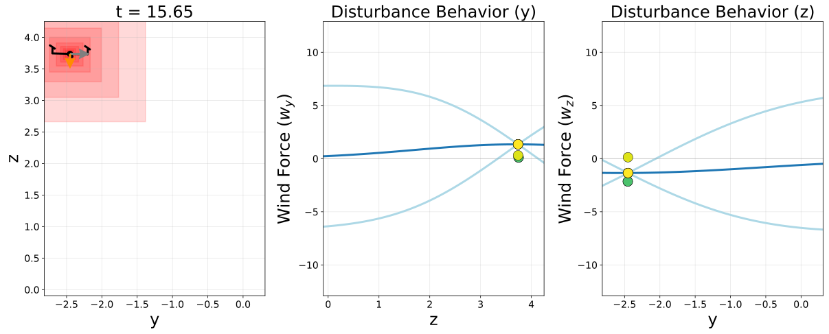
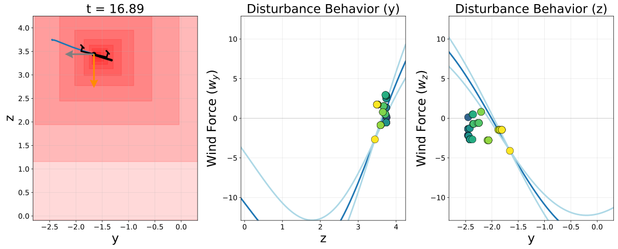
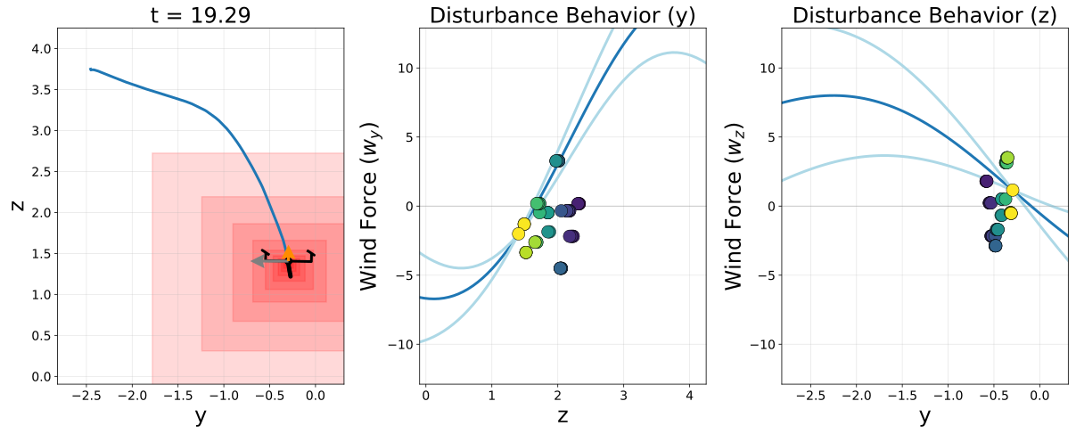
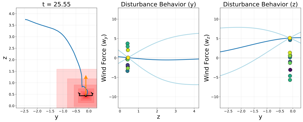
MM-GPR tube rejects an unmodeled industrial-fan disturbance. With GP estimation disabled, tubes become inaccurate and the mission fails[6]
NRT inside a runtime-assurance framework using forward-invariant tubes around reference trajectories:
Disturbances estimated online via time-varying Gaussian processes
Replanning triggered when tube can no longer certify safety
NRT at 100 Hz, immrax[7] tube updates at 10 Hz — full pipeline meets 10 ms budget on average
Thrust 1 — Takeaways
Summary of Thrust 1
NRT method occupies a valuable middle ground between high-accuracy control and efficient compute
Modular implementation with minimal tuning
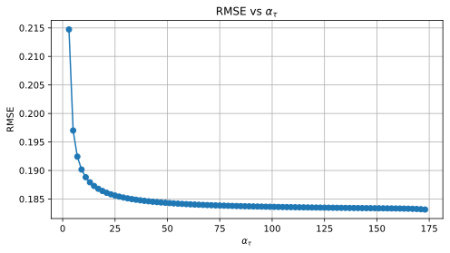
\(\alpha\)-stability proof on the linearized miniature blimp; empirically near-insensitive to \(\alpha\) over a broad plateau
Deployed on real hardware (blimp, quadrotor) with high accuracy, fast computation time, and low-energy footprint
Efficiency leaves time and compute for high-level tasks; demonstrated in I-STL and GP invariant tube work
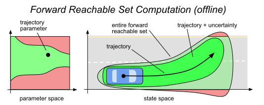
Offline FRS computation: each trajectory parameter \(k\) (left, parameter space) maps to a trajectory plus uncertainty tube inside the entire forward reachable set (right, state space). Reproduced from [8].
Reachability-based Trajectory Design (RTD) Core
Planning model. Low-fidelity model used for FRS computation offline; worst-case tracking-error inflation absorbs model mismatch.
Offline FRS. Trajectories parameterized by \(k\).
Online Optimization.\(k^\star=\arg\min_{k\in K_{\mathrm{adm}}} J(k)\ \ \text{s.t. } k \text{ is obstacle-free}\)
Offline FRS computation: each trajectory parameter \(k\) (left, parameter space) maps to a trajectory plus uncertainty tube inside the entire forward reachable set (right, state space). Reproduced from [8].
Reachability-based Trajectory Design (RTD) Core
Planning model. Low-fidelity model used for FRS computation offline; worst-case tracking-error inflation absorbs model mismatch.
Offline FRS. Trajectories parameterized by \(k\).
Online Optimization.\(k^\star=\arg\min_{k\in K_{\mathrm{adm}}} J(k)\ \ \text{s.t. } k \text{ is obstacle-free}\)
Offline FRS computation: each trajectory parameter \(k\) (left, parameter space) maps to a trajectory plus uncertainty tube inside the entire forward reachable set (right, state space). Reproduced from [8].
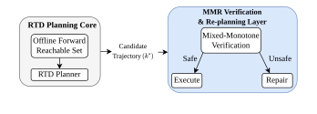
Departure: strip the offline FRS of its tracking-error inflation and delegate safety certification to the online MMR verifier against the measured disturbance. First RTD-class framework to safely plan under a priori unknown disturbances.
Why Mixed-Monotone Reachability
Embedding trajectory and reachable tube under bounded disturbance \(w\in[-1,1]\).
MMR enables efficient calculation of hyperrectangular reachable set overapproximations via a single ODE integration. immrax[7] provides an embedding system for our dynamics and JIT-compiles it for real-time reachability.
Case Study 1 — Narrow Gap
Animated side-by-side: Standard RTD (left) remains infeasible through the gap; RTD-RAX (right) uses the non-inflated FRS plus immrax verification to certify a safe corridor path.
Two rectangular obstacles make a narrow gap:
Standard RTD: inflated FRS declares infeasible → fail-safe triggered
RTD-RAX: optimizer returns \(k^\star\) through the gap → mixed-monotone tube certifies safe
Scenario isolates the effect of offline FRS conservatism
Case Study 2 — Angled Obstacle
At each step: generate candidate → verify → execute or repair.
Standard RTD succeeds conservatively
RTD-RAX: rejections become repaired candidates via speed-backoff + buffer tightening → shorter, more efficient paths
Side-by-side animation: Standard RTD (conservative but succeeds) and RTD-RAX (online verification + repair reaches goal).
The RTD-RAX path is shorter than the Standard RTD path.
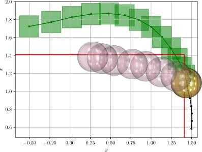
Close-up of two repair events: unsafe candidate tube (pink) rejected, repaired tube (green) chosen and executed. Animation pauses at each repair for visual clarity.
Case Study 3 — Unknown Disturbances
Multi-gap course with disturbance patches. Top: Standard RTD collides on cycle 3. Bottom: RTD-RAX senses, verifies, repairs, and reaches the goal.
The verifier + repair layer turns mission failures into safe alternatives.
Verification and simple repairs often happen near-instantly: trade \(\approx\!1\) ms online compute for a recovered, certifiably safe path
Receding-horizon with multiple disturbance patches.
Planner
Outcome
Cycles
Repairs
Mean / p95 [ms]
Std RTD
Collision
3
—
10.5 / 21.9
RTD-RAX
Goal reached
19
3
10.5 / 37.4
Mean unchanged — verification is flat on typical cycles.
p95 tail isolates the repair loop’s worst-case cost.
First RTD-class framework to certify safety under a priori unknown runtime disturbances [9].
Thrust 2 — Takeaways
Summary of Thrust 2
RTD-RAX separates fast candidate generation from execution-time safety certification.
Uses MMR with measured disturbance bounds online — first RTD-class method accommodating a priori unknown disturbances.
Verification adds negligible added mean cycle time; adds cost on the p95 tail when many repairs fire.
Repair layer turns rejections into safe alternatives before falling back to a certified fail-safe.
Feed disturbance measurements back into core RTD program as constraints and/or warm-start with disturbance-aware repaired trajectory parameters. \[
\min_k \, J(k) \; \text{s.t. } k \text{ is obstacle-free},\;\; k_0 = k^{\text{wind}}
\]
P2.2 — Learned GP Disturbance Bounds
Current. Simulated disturbance known at every iteration.
Learn the disturbance online from a measured residual between estimated acceleration and measured acceleration.
Pay-off. Learns from flight data.
More recent measurements weighted more strongly. SITL precedent in gale-force conditions. Hardware precedent in IFL against an industrial fan.
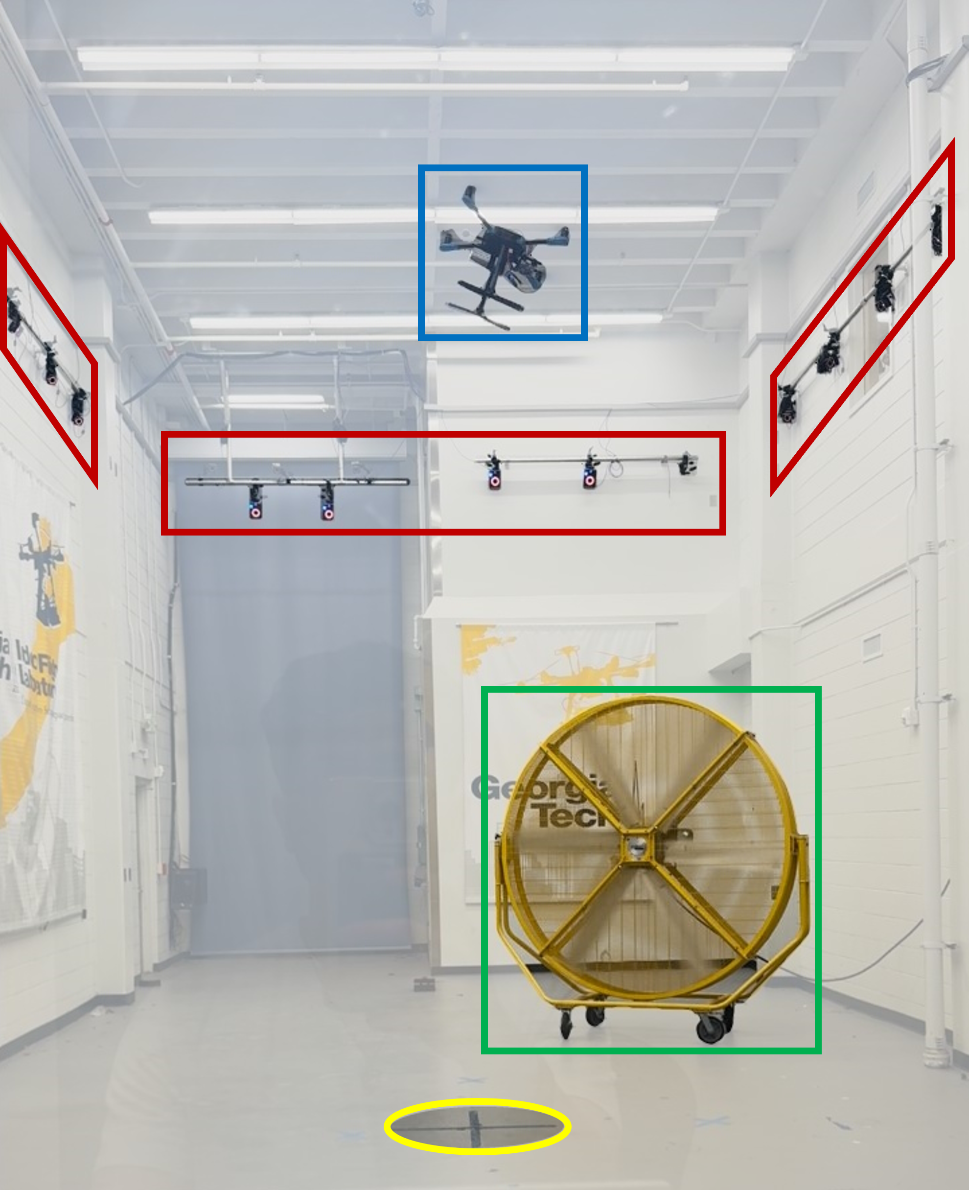
Setup for hardware experiments in the Indoor Flight Lab at Georgia Tech. The quadrotor (blue), tracked by a motion capture system (red), landing pad (yellow), while in the presence of wind created by an industrial fan (green).
P2.3 — Hardware Validation
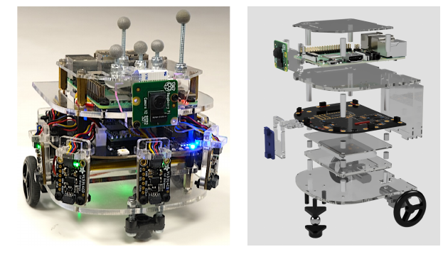
Step 1: GTernal ground robot — port simulation case studies, characterize real disturbances, validate repair online
Extend from spatial safety to full STL mission specifications by learning which parameters map onto given STL formulas:
Offline. Learn mapping between trajectory parameter space and specification-observing trajectories.
Online. Use this map instead of core RTD optimization until robustness falls below desired value, or higher-level safety concerns become more important
MMR verifier always ensures safety vis-a-vis obstacles with disturbance-awareness
What STL adds beyond “avoid obstacles”: timed, sequenced, conditional objectives.
Reach\(G\) by \(T\): \(\Diamond_{[0,T]}(x{\in}G)\)
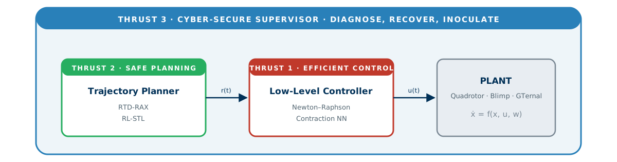
Failure-Mode Inoculation. Accumulate verified safety-preserving strategies for each fault class so recurring faults are handled faster each time.
STEP 1
Diagnose
Real-time root-cause isolation of the anomaly.
→
STEP 2
Recover
Online recovery into a safe operating regime.
→
STEP 3
Inoculate
Accumulate verified safety-preserving strategies for each fault class so recurring faults are handled faster each time
Like a biological immune response, each new attack expands the resilient operating envelope.
P3.1 — System parameter → Safe-Strategy Map
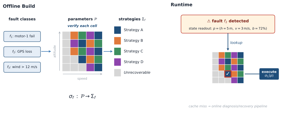
For each fault class \(f\), precompute an offline map \[\sigma_f : \mathcal{P} \to \Sigma_f\] from system parameters \(p \in \mathcal{P}\) (altitude, speed, battery) to a pre-certified backup strategy.
Offline sweep: Verify regions \((f, p)\) that can be salvageable via backup strategies
Runtime: Simple lookup/mapping → execute on the certified strategy
Coverage guarantee: if \((f,p)\) is in the sampled grid, the strategy is certified by construction
Outside the grid: fall back to the online inoculation pipeline
P3.1 broadly classifies (fault, parameters) into a backup-strategy class; we now turn these into an actual recovery strategy
Instead of executing a one-size-fits-all re-stabilizing backup, each class carries a cached warm-start that seeds an online optimal-recovery program — precomputed templates refined online, rather than cold-solved from scratch.
Offline build. For each fault class \(f\), encode the safe-recovery strategy. Sweep the parameter grid \(\mathcal{P}\) and cache the optimal recovery trajectory \(z^\star_f(p)\) as a warm-start.
Runtime trigger. Fault \(f\) at parameters \(p\) → retrieve \(z^\star_f(p)\) from the cache → warm-start the online optimal-recovery program → much faster feasible recovery instead of cold-solve latency.
If no such backup strategy exists in the cache for the current (fault, parameters), fall back into a broader diagnosis/recovery pipeline.
Conclusion
Wrapping Up
1Completed publications2Proposed research timeline3Closing remarks
Plan of Work — Completed
Venue
Milestone
Status
ACC
First hardware validation of NRT on quadrotor
Published
TCST
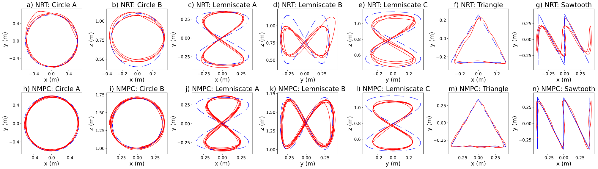
Competitive tracking performance shown on quad and blimp vs NMPC, FBL
Accepted
NAHS
I-STL runtime assurance on blimp with NRT method as LLC + \(\alpha\)-stability proof for blimp
In revision
MECC + ALDSC Joint Submission
RTD-RAX Architecture
Submitted
OJ-CSYS
GP-tube tracking, quadrotor validation + NRT Method as LLC
Submitted
Plan of Work — Proposed
Term
Milestone
Summer 2026
Contraction-NN tracker on Holybro X500 vs NRT/NMPC (P1.1, CoRL)
Summer 2026
RTD-RAX: GP disturbance bounds + gradient repair (P2.1–P2.2)
Fall 2026
RL-STL MILP-on-trigger policy (P2.5)
Fall 2026
RTD-RAX hardware: GTernal → Holybro X500 (P2.3)
Spring 2027
Parameter → STL trajectory map (P2.4)
Spring 2027
Certified backup-controller library, one fault class (P3.1)
M. E. Cao, A. Harapanahalli, E. Morales-Cuadrado and S. Coogan, “Trajectory Tracking for Systems with Unknown Time-Varying Disturbance,”IEEE OJ-CSYS (submitted), 2026.
Thank You
Computationally Efficient and Safe Control for Aerial Robotic Systems under Threat and Disturbance
A research program for efficient, robust, and cyber-secure autonomy.
All hardware uses OptiTrack / Vicon for motion capture
PX4-based quadrotor fuses MoCap with onboard sensors via the PX4 EKF2 [5].
Backup. Tooling Stack
JAX (forward-mode autodiff, JIT) — nonlinear predictors and Jacobians for the NRT flow on the quadrotor [5]
immrax[7] — automated embedding-system construction and MMR propagation
acados — NMPC baseline (SQP-RTI with computational-delay compensation)[5]
Gurobi (MILP) — I-STL plan synthesis at 2 Hz; NRT runs the 50 Hz low-level loop [4]
PX4/ROS2 — EKF2 estimator, ROS 2 / \(\mu\)XRCE-DDS middleware, cascaded-PID native baseline and real-time messaging on the quadrotor [1]
Gazebo + PX4 SITL — GP-tube validation with controllable wind fields up to 17 m/s [6]
Backup. Quadrotor — Dynamic Model
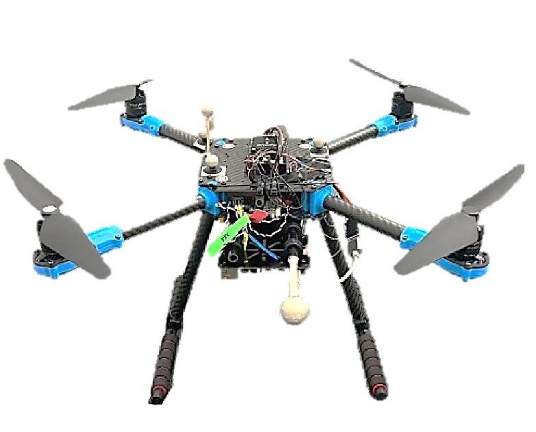
9-state, 4-input nonlinear model used for the Holybro X500 V2 hardware [5]. State \(x=[p_x,p_y,p_z,\;V_x,V_y,V_z,\;\phi,\theta,\psi]^\top\in\mathbb R^9\); input \(u=[u_\tau,\;u_p,u_q,u_r]^\top\in\mathbb R^4\) (net thrust + body rates).
where \(T_\Theta\) is the Euler-rate transformation matrix.
Tracked output \(y=(p_x,p_y,p_z,\psi)^\top\in\mathbb R^4\) — input/output dimensions match (\(m{=}p{=}4\)), so \(\partial_u\rho\) is square [5]
NRT predictor uses RK4 integration of the above from \((x(t),u(t))\) held constant over \([t, t+T]\)
\(\partial_u\rho\) via JAX forward-mode autodiff
Backup. Blimp — Nonlinear Dynamics
GT-MAB platform[13]: radially-symmetric blimp with undermounted gondola; CG sits below the center of buoyancy along body \(\hat z\) at offset \(r^b_{z,g/b}\)
State\(x=(\nu^b_{b/n},\eta^n_{b/n})\in\mathbb R^{12}\) with \(\nu^b\) = body-frame translational/angular velocities and \(\eta^n\) = world-frame position + Euler angles
with mass/inertia \(M^{CB}\), Coriolis \(C^{CB}(x)\), aerodynamic damping \(D^{CB}\), restoring gravity \(G^{CB}(x)\), and constant input map \(L\in\mathbb R^{6\times 4}\).
Buoyancy cancels translational gravitational acceleration; the CB–CG offset induces a non-zero roll/pitch restoring torque.
Backup. Blimp — Hover Linearization
Underactuation[13, Eq. 2]: the 4-D input \(u\) maps into a 6-D wrench via \(\tau^b = L u\) with constant \(L\in\mathbb R^{6\times 4}\)
Operating point: level hover with \(\nu^b=0\), \(\Theta^n=0\). Linearizing the GT-MAB model about this point preserves the underactuation through \(B\):
\[\dot x \;=\; A\,x + B\,u, \qquad B = (M^{CB})^{-1}\,L, \qquad (A,B) \text{ constant.}\]
Trade-off: valid only while \(\|\Theta\|\) stays small; aggressive attitude maneuvers push the linearization into model-mismatch territory.
Memoryless plant\(y(t)=g(u(t))\); seek \(u\) such that \(g(u)=r\). Discretize with step \(\Delta t\), \(t_k=k\Delta t\): \[u(t_{k+1}) \;=\; u(t_k) + \Delta t\,\Bigl(\tfrac{\partial g}{\partial u}(u(t_k))\Bigr)^{-1}\bigl(r(t_k)-g(u(t_k))\bigr).\]
Rearrange as a difference quotient and take the limit\(\Delta t\to 0\) to obtain the continuous-time NRT flow; scaling by a speedup factor\(\alpha>1\) yields [2]: \[\boxed{\;\dot u(t) = \alpha\,\Bigl(\tfrac{\partial g}{\partial u}(u(t))\Bigr)^{-1}\bigl(r(t)-g(u(t))\bigr)\;}\qquad\limsup_{t\to\infty}\|r(t)-y(t)\|\;\leq\;\alpha^{-1}\limsup_{t\to\infty}\|\dot r(t)\|.\]
T1 Backup. NRT — Dynamical-Systems Case
Problem Given \(\dot x = f(x,u)\), \(y = h(x)\) — there is no static map \(u\mapsto y\); the output depends on the trajectory of \(u\), and the system dynamics not just its instantaneous value.
Resolution[2]: replace \(g(u(t))\) with a ZOH look-ahead predictor\(\hat y(t+T)=\rho(x(t),u(t))\) — the predicted output \(T\) seconds ahead assuming the current \(u\) stays frozen (construction on the next slide). Substituting \(g\to\rho\) and shifting the reference \(r(t)\to r(t+T)\) in the memoryless NRT flow yields:
Asymptotic error bound[2, Thm. 4.5]:\(\limsup_{t\to\infty}\lVert r(t)-y(t)\rVert \,\leq\, \nu_1+\nu_2/\alpha\), where \(\nu_1\) accounts for prediction inaccuacy over horizon \(T\) and \(\nu_2\) for reference speed \(\lVert\dot r\rVert_\infty\)
\(\alpha\) is a speedup, not a gain — it multiplies \(\dot u\), not \(u\)
T1 Backup. NRT — ZOH Predictor
ZOH assumption[2]: hold \(u\) constant over \(\tau \in [t, t+T]\) and define \[
\rho(x(t),u(t)) \;\triangleq\; C\,x(t+T)\;\big|_{\dot x = f(x,u(t)),\; x(t)=x(t),\; u(\tau)=u(t)}
\]
This is the (model-predicted) output at the lookahead horizon \(t+T\) assuming the current \(u\) stays frozen.
Linearized case. Closed-form: \[
\begin{aligned}
\rho(x,u) &= C e^{AT}x + C\!\int_0^T e^{As}\mathrm ds\,B\,u \\
&=: C\tilde A x + C\tilde B u
\end{aligned}
\] → constant Jacobian \(J=C\tilde B\)[5]
Nonlinear case.\(\rho\) via numerical integration:
RK4/Euler: \(\partial_u\rho\) via autodiff or finite differences [12]
Horizon \(T\) is a tuning knob: small \(T\) → high-frequency noise; large \(T\) → stale prediction.
T1 Backup. NRT — \(\alpha\)-Stability Definition
Definition 4.1[2]. The NRT-closed-loop system is \(\alpha\)-stable on a compact set \(\Gamma\subset\mathbb R^{n+m}\) if \(\exists\,\bar\alpha\geq 0\) and class-\(\mathcal K\) functions \(\beta,\gamma_1,\gamma_2\) such that for every \(z(0)\in\Gamma\), every bounded reference \(r\) with bounded \(\dot r\), and every \(\alpha\geq\bar\alpha\), \[\lVert z(t)\rVert \leq \beta(\lVert z(0)\rVert) + \gamma_1(\lVert r\rVert_\infty) + \gamma_2(\lVert\dot r\rVert_\infty).\]
Intuition. The extended state \((x,u)\) stays bounded by three additive budgets: a transient from the initial condition, a tax for reference magnitude, and a tax for reference speed.
Key property: the bounds hold uniformly in \(\alpha\) once \(\alpha\geq\bar\alpha\) — increasing the gain never destabilises. By Proposition 4.2 of [2], \(\alpha\)-stability implies\(\lim_{\alpha\to\infty}\limsup_t\lVert r-\hat y\rVert=0\) for references with \(\dot r\to 0\). This is the BIBS-with-speedup variant; distinct from standard ISS in that \(\alpha\) appears as a control parameter, not a fixed gain [2].
T1 Backup. NRT — Convergence Bound Derivation
Corollary 3.5 of[2]. For any bounded reference with bounded derivative, the tracking error of the NRT flow satisfies \[\limsup_{t\to\infty}\lVert r(t)-y(t)\rVert \;\leq\; \eta_1 + \tfrac{\eta_2}{\alpha}.\]
\(\eta_1\) — sup-norm of the prediction-model residual\(\lVert\rho(x(t),u(t)) - y(t+T)\rVert\); vanishes only if \(\rho\) matches the true ZOH output exactly. Floor that \(\alpha\) cannot touch.
\(\eta_2\) — proportional to \(\sup_t\lVert\dot r(t+T)\rVert\), the reference’s own rate of change; attenuated by \(1/\alpha\) because larger \(\alpha\) tracks the moving target faster.
T1 Backup. NRT — iCBF Mechanism Sketch
The NRT dynamic law \(\dot u = \phi(x,u,t)\) is augmented with a min-norm perturbation \(v\in\mathbb R^m\) to enforce safety on the augmented set \(\mathcal S=\{(x,u)\in\mathbb R^{n+m}:h(x,u)\geq 0\}\)[3, Thm. 1]:
\[\dot u \;=\; \phi(x,u,t) + v^\star,\qquad v^\star \;=\; \operatorname{arg\,min}_{v\in\mathbb R^m}\;\tfrac{1}{2}\lVert v\rVert^2 \quad\text{s.t.}\quad p(x,u)^\top v \;\geq\; d(x,u,t),\]
with \(p(x,u)\!:=\!(\partial_u h)^\top\) and \(d(x,u,t)\!:=\!-\bigl[\partial_x h\,f(x,u)+\partial_u h\,\phi(x,u,t)+\gamma(h(x,u))\bigr]\).
I-CBF condition[3, Def. 1]: \(p(x,u)=0 \Rightarrow d(x,u,t)\leq 0\) — qualifies \(h\) as an I-CBF and guarantees QP feasibility
Single affine inequality + quadratic cost → min-norm closed form\(v^\star = \bigl(d/\lVert p\rVert^2\bigr)\,p\) if \(d>0\), else \(0\)[3, Eq. 19]
Holds even when \(f(x,u)\) is not control-affine
Can encode input bounds
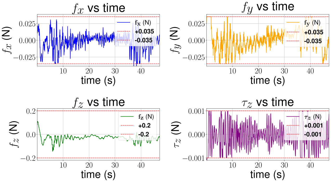
Input bounds are I-CBFs too:\(h(u)=u_{\max}^2-\lVert u\rVert^2\) satisfies the I-CBF condition [3, Lem. 1], so \(u\) is kept in-envelope by integration of \(\dot u=\phi+v^\star\) rather than by hard saturation — no windup.
T1 Backup. NRT — Flat-Domain Predictor
The quadrotor is differentially flat in \(\sigma=[x,y,z,\psi]^\top\): the full state and input are recovered algebraically from \(\sigma\) and its derivatives up to order \(\ell=3\)\[
x=\beta(\sigma,\dot\sigma,\ddot\sigma,\dddot\sigma),\qquad u=\Phi(\sigma,\dot\sigma,\ddot\sigma,\dddot\sigma).
\] NRT is then run in the flat domain with flat state \(x_\mathrm{flat}=[\sigma,\dot\sigma]\) and flat input \(u_\mathrm{flat}=\ddot\sigma\) — one derivative below the order needed by \(\Phi\), so the NRT update naturally produces the jerk \(\dddot\sigma_\mathrm{des}\).
Jacobian inverse is a constant scalar — no matrix factorization per step. Flat-domain law: \[
\dddot\sigma_\mathrm{des} \;=\; \alpha\odot\bigl(\tfrac{2}{T^2}\,I_4\bigr)\bigl(r(t{+}T)-\rho\bigr).
\]
A triple-integrator chain \(\dot z = A_3 z + B_3\,\dddot\sigma_\mathrm{des}\) with \(z=[\sigma,\dot\sigma,\ddot\sigma]^\top\) is forward-Euler integrated each tick to recover \(\chi=[\sigma,\dot\sigma,\ddot\sigma,\dddot\sigma]_\mathrm{des}\), then \(\Phi(\chi)\) produces \(u_\mathrm{des}=[F,p,q,r]\) on the PX4 inner loop.
Implementation (JAX, JIT)
12-D flat state x_df = [σ, σ̇, σ̈], control u_df = σ⃛
\(\Phi\) done explicitly: thrust \(=m\lVert\ddot\sigma+g\hat z\rVert\); body axes built from \(\hat b_3\) + yaw heading; body rates \((p,q)\) projected from jerk; yaw-rate \(r\) algebraically solved
T1 Backup. TCST — NMPC Formulation
Error-state OCP — state \(x=[p,v,\eta]\in\mathbb R^9\), input \(u=[F,p,q,r]\in\mathbb R^4\) (collective thrust + body rates) [5]: \[
\min_{x_{0:N},\,u_{0:N-1}}\; \tfrac{1}{2}\|e_N\|_{Q_e}^2 + \tfrac{1}{2}\sum_{k=0}^{N-1}\|e_k\|_W^2
\;\;\text{s.t.}\;\; x_{k+1}=\Phi_{\!\Delta t}(x_k,u_k),\;\; x_0=\hat x(t),\;\; u_k\in\mathcal U,
\] where \(e_k=[\,p_k-p_k^\mathrm{ref},\,v_k-v_k^\mathrm{ref},\,\mathrm{atan2}(\sin\Delta\psi,\cos\Delta\psi),\,u_k-u_k^\mathrm{ref}\,]\) uses wrapped yaw error
Real-time iteration in acados
nlp_solver = SQP_RTI — one SQP iteration per control step, no convergence loop
cost_type = NONLINEAR_LS with stage-wise reference parameter \(p_k=[p^\mathrm{ref},v^\mathrm{ref},\eta^\mathrm{ref},u^\mathrm{ref}]\in\mathbb R^{13}\) — references enter as parameters, not via yref rebuild
Two 100 Hz ROS timers ride out solve-time jitter without per-step latency:
compute_control_timer (100 Hz): solves the OCP, warm-starts \(u_0\!\leftarrow\!u_\mathrm{last}\), writes the full\(N\)-step input plan into control_buffer and resets buffer_index=0
publish_control_timer (100 Hz): accounts for computation delay and uses the appropriate \(n^{th}\) input
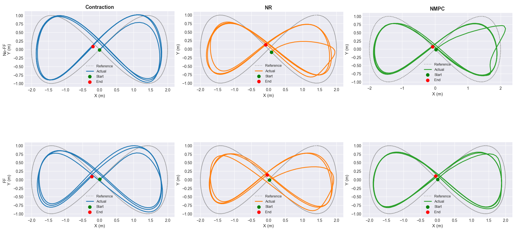
With differential-flatness feedforward (--ff, used in the contraction study), per-stage references include flat-output-derived \(\eta^\mathrm{ref}_k\) and \(u^\mathrm{ref}_k\) instead of hover — the SQP step then only solves for the residual correction, sharply reducing transient excursions.
Input-output FBL for the GT-MAB blimp [13, Thm. 1]: with output \(\sigma=[x,y,z,\psi]^\top\), each channel has relative degree 2 (away from \(\theta,\phi=\pm\pi/2\)), so \(\ddot\sigma = A(x) + B(x)u\).
Invert the input map and solve for virtual input \(q\in\mathbb R^4\): \[
u(x) = B(x)^{-1}\bigl(q - A(x)\bigr), \qquad q = \ddot r + K_d(\dot r - \dot y) + K_p(r - y)
\] giving linear residual dynamics \(\ddot e + K_d\dot e + K_p e = 0\) on tracking error \(e=\sigma-r\).
Requires reference derivatives \((\dot r, \ddot r)\) — same as NMPC, unlike NRT
4-D zero dynamics in \((\phi,\theta,\omega^b_x,\omega^b_y)\) are only lightly damped under realistic GT-MAB inertias [13, Lem. 1, Thm. 2] → mitigated in [13] by an HOCBF QP capping \(|\phi|,|\theta|\)
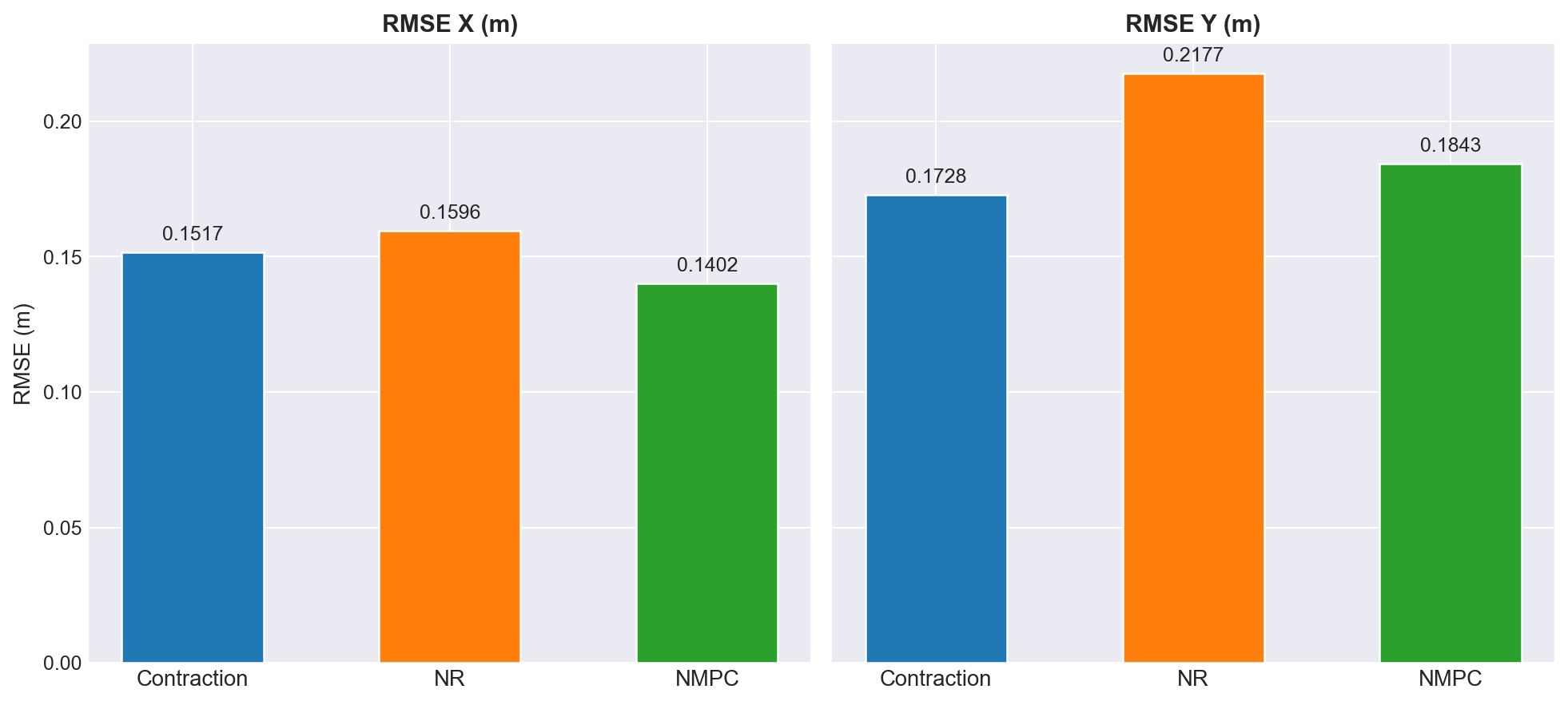
“Clipped” removes the initial hover-to-reference transient; “With Transients” includes it.
RMSE [m] — Clipped vs. With Transients
Trajectory
NRT Clipped
NMPC Clipped
NRT Full
NMPC Full
Circle A
0.10695
0.03932
0.12266
0.10653
Circle B
0.11887
0.03246
0.12276
0.15162
Lemniscate A
0.12328
0.09738
0.12249
0.11311
Lemniscate B
0.15915
0.04683
0.15203
0.10479
Lemniscate C
0.14554
0.09938
0.14532
0.17329
Helix A
0.14879
0.13327
0.14867
0.16865
Helix B
0.19540
0.14977
0.18851
0.18044
Circle C
0.17398
0.14782
0.17073
0.17715
Sawtooth
0.04014
0.02331
0.04505
0.06032
Triangle
0.05979
0.01803
0.08136
0.08387
Per-iteration compute [ms]
Trajectory
NRT
NMPC
Circle A
2.381 ± 0.206
13.036 ± 0.173
Circle B
2.426 ± 0.201
13.352 ± 0.139
Lemniscate A
2.438 ± 0.239
13.088 ± 0.092
Lemniscate B
2.486 ± 0.200
13.288 ± 0.246
Lemniscate C
2.397 ± 0.200
9.216 ± 5.646
Helix A
2.480 ± 0.222
13.307 ± 0.196
Helix B
2.471 ± 0.271
13.294 ± 0.110
Circle C
2.454 ± 0.255
13.705 ± 0.222
Sawtooth
2.507 ± 0.254
13.329 ± 0.140
Triangle
2.417 ± 0.196
13.182 ± 0.291
Bold = winner per category. NRT consistently ~5.3–5.6\(\times\) faster than NMPC per iteration.
T1 Backup. TCST Results — Blimp
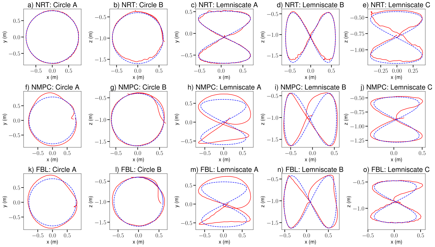
Newton-Raphson tracker (NRT) vs. NMPC vs. FBL on the miniature blimp [5].
NRT receives no reference-derivative information; NMPC and FBL are given \(\dot r\).
Bold = winner per category
RMSE [m] — standard + aggressive trajectories
Trajectory
NRT
NMPC
FBL
Circle A
0.079
0.141
0.193
Circle B
0.051
0.110
0.143
Lemniscate A
0.104
0.185
0.230
Lemniscate B
0.054
0.103
0.146
Lemniscate C
0.056
0.118
0.131
Helix A
0.072
0.077
0.113
Helix B
0.088
0.215
0.220
Circle C
0.101
0.403
0.384
Per-iteration compute [ms]
Trajectory
NRT
NMPC
FBL
Circle A
0.84 ± 0.05
58.7 ± 15.7
10.4 ± 9.7
Circle B
0.82 ± 0.03
51.5 ± 12.2
10.9 ± 10.4
Lemniscate A
0.82 ± 0.02
52.7 ± 12.5
10.5 ± 10.7
Lemniscate B
0.87 ± 0.23
54.2 ± 6.8
10.8 ± 10.1
Lemniscate C
0.86 ± 0.02
54.8 ± 11.9
10.7 ± 10.4
Helix A
0.94 ± 0.04
53.2 ± 6.8
9.9 ± 9.5
Helix B
0.95 ± 0.02
60.8 ± 12.8
10.3 ± 10.1
Circle C
0.96 ± 0.03
73.5 ± 20.9
10.2 ± 9.9
NMPC misses the 25 ms control deadline on every trajectory → degraded tracking.
NRT is ~10× faster than FBL and ~60× faster than NMPC on this platform.
T1 Backup. I-STL RTA — Problem & Why I-STL
Setting[4]: linear discrete-time system \(x_{k+1}=Ax_k+Bu_k+Gw_k\), \(w_k\in\mathcal W\) bounded, plus a (possibly unsafe) nominal controller\(\hat u\) and a bounded-horizon Interval STL safety formula \(\varphi\) with affine predicates \([\alpha]^\top[x]-[\beta]\geq 0\).
Goal: at every time \(t\), output \(u_t\) that minimally deviates from \(\hat u_t\) while guaranteeing \(\underline\rho^\varphi(\mathbf x,k)\geq 0\) for all\(k\geq 0\) and all disturbance realizations.
Why I-STL (vs. plain STL)?
Standard STL evaluates a single deterministic trajectory; under disturbance \(w\in\mathcal W\) you’d need a separate proof for every realization
I-STL evaluates robustness over interval-valued signals \([\mathbf x]\), so disturbance reachable sets propagate natively through the temporal operators
Soundness [4, Prop. 1]:\(\underline\rho^\varphi([\mathbf x],t)\geq 0\;\Rightarrow\;\rho^{\varphi'}(\mathbf x,t)\geq 0\;\forall\,\mathbf x\in[\mathbf x]\) — one MIP solve certifies every realization
Receding-horizon RTA program[4, Eq. 7]: \[
\begin{aligned}
\min_{\,u_t,\dots,u_{t+N-1}}\;& \max_{w\in\mathcal W}\,\|\hat u_t - u_t\|\\
\text{s.t. }& x_{k+1}=Ax_k+Bu_k+Gw_k\\
& \underline\rho^\varphi(\mathbf x,k)\geq 0\\
& u_k\in\mathcal U
\end{aligned}
\] Encoded as a MILP via stlpy extended with npinterval for I-STL semantics — integer variables enforce the temporal-operator big-M constraints exactly.
Three obstacles to making this real-time — (1) recursive feasibility under disturbance, (2) the inner \(\max\) over \(w\), (3) MIP solve too slow for low-level control. Each is addressed on the next slide.
Recursive feasibility [§ V]: terminal constraint \([x]_{t+N-\|\varphi\|:t+N-\|\varphi\|+b-1}\!\subseteq\!\mathcal S\), where \(\mathcal S\!\subseteq\!(\mathbb R^n)^b\) is the persistently feasible set — strictly more conservative than the (intractable) maximal RCI in the language space \(\mathcal L(\varphi)\), but computable. Built once offline via robust controllable sets [Prop. 2] using polytope/zonotope ops (cddlib, pypoman).
Tube MPC for \(\max_w\) [§ VI]: replace the inner max with interval-valued state propagation \([x]_k = x_k + [Z](k\!-\!t)\) and a tightened input set\(\mathcal U \ominus K Z(k\!-\!t)\); closed form, no nested optimization.
Slack variable [§ VII]: relax \(\underline\rho^\varphi\geq 0 \,\to\, \underline\rho^\varphi\geq -\xi\), \(\xi\geq 0\), with high cost \(\gamma^\top\xi\) — gives graceful degradation when the sim-to-real residual exceeds \(\mathcal W\) (in reported runs \(\xi\equiv 0\)).
Warm-start across MIP instances [§ IX]: shift the previous solution by one step to seed the next solve.
Newton-Raphson tracker[2] follows the spline on the host (Dell laptop) — asymptotic residual error \(\eta_1+\eta_2/\alpha\)
Deadline-miss safe by construction: the previous backup trajectory’s tail still terminates in \(\mathcal S\) → executing its next step preserves \(\underline\rho\geq 0\) under worst-case \(\mathcal W\) — no manual intervention needed
The split decouples correctness (slow MIP, I-STL interval semantics) from bandwidth (fast NRT tracking the spline).
T1 Backup. I-STL RTA — Blimp Hardware Validation
Platform[4]: GT-MAB 6-DOF miniature blimp, hardware in real time. Dynamics linearized about hover for the RTA MIP; nonlinear in the NRT tracking layer. Nominal PID loops four corners of \(\mathcal S\) → violates both specs by construction.
Specs — central square \(\mathcal S\), side \(\approx 2.82\) m
\(\vartheta = (x\in\mathcal S)\Rightarrow \diamondsuit_{[0,4]}(x\notin\mathcal S)\) — exit within 4 s of entry
\(\varphi = (x\in\mathcal S)\Rightarrow \diamondsuit_{[0,3]}\Box_{[0,1]}(x\notin\mathcal S)\) — same plus a nested 1 s dwell-out
Sim: RTA never missed its 0.5 s deadline; \(\underline\rho^\varphi\geq 0\) throughout both runs
Hardware: deadline missed $\(1\)$/50 s — safety preserved automatically by the previous backup; no falls into \(\mathcal S\)
Both specs satisfied across the entire run; the nominal PID violation pattern is bent into a verified safe trajectory
First hardware demo of I-STL RTA on the GT-MAB platform: linearized 12-D blimp model in the RTA MIP, full 6-DOF nonlinear model in the NRT tracking layer — prior I-STL control synthesis was simulation-only on a linearized model
The persistent-feasibility net is the design payoff: occasional MIP overruns, which would chatter or crash a simplex-style RTA, are absorbed silently — the system is provably safe even when the optimizer fails.
T1 Backup. GP-Tube — Runtime Trigger
For \(\dot x=f(x,u,w)\) with \(w\!=\!g(t,x)\) unknown, [6] build a forward-invariant tube of radius \(\varepsilon\) around the reference \(x_r(t)\) by:
modelling \(g\) as a time-varying Gaussian process
using mixed-Jacobian inclusion to construct an embedding system
propagating \([\underline x(t),\overline x(t)]\) alongside \(x_r\) under the tracking controller.
Mechanism: Identify the earliest time \(t^\star\) at which the tube can no longer stay inside the \(\varepsilon\)-neighborhood of \(x_r\).
At \(t^\star\), trigger:
Collect a fresh \(g\) sample
Update the GP
Recompute reference + tube
Identify the next \(t^\star\)
Full pipeline in ~0.11 ms mean, tube-recompute at 100 Hz body-rate loop without missing deadlines.
Same Holybro X500 V2 used for NRT-vs-NMPC study [5]
Indoor industrial fan to produce wind
Same tube propagation as in SITL; directly portable to hardware from simulation results
T1 Backup. GP-Tube — SITL Computation Budget
Computation
Average [ms]
Max [ms]
Joint NRT + LQR controller
\(0.0026 \pm 0.00069\)
0.00677
Invariant tube (mixed-Jacobian inclusion)
\(0.108 \pm 0.0059\)
0.134
Body-rate commands at ~100 Hz → full pipeline inside 10 ms
Tube computation triggered intermittently (when tube approaches \(\varepsilon\)-boundary), not per control step
Enabled by JAX JIT compilation and immrax[7] automated inclusion-function construction
Simulated wind magnitudes up to ~17 m/s (near gale-force) — well beyond what even industrial fans can reproduce [6]
T1 Backup. GP-Tube — GP Basics
A Gaussian process (GP)[6] is a distribution over functions \(g:\mathbb R^n\to\mathbb R\) such that any finite set of evaluations \(\{g(x_1),\dots,g(x_\tau)\}\) is jointly Gaussian, fully specified by a mean function \(m(x)\) (here taken as zero) and a covariance kernel \(k(x,x')\).
Posterior given \(\tau\) noisy observations\(y_j=g(x_j)+\varepsilon_j,\;\varepsilon_j\sim\mathcal N(0,\sigma^2)\): \[
\begin{aligned}
\mu_\tau(x) &= k_\tau(x)^\top(K_\tau+\sigma^2 I)^{-1}y_\tau\\[-2pt]
\sigma_\tau^2(x) &= k(x,x)-k_\tau(x)^\top(K_\tau+\sigma^2 I)^{-1}k_\tau(x)
\end{aligned}
\] where \(k_\tau(x)=(k(x_1,x),\dots,k(x_\tau,x))^\top\) and \(K_\tau=[k(x_i,x_j)]\).
The mean \(\mu_\tau\) is the best-guess function; the variance \(\sigma_\tau^2\) is the uncertainty in that guess at \(x\).
Why GPs (vs. point estimates)
Calibrated uncertainty — a probabilistic envelope on the guess
Tightens with data — \(\sigma_\tau^2(x)\to 0\) as observations cluster near \(x\)
Kernel-driven smoothness prior — encodes “nearby inputs ⇒ nearby outputs” without picking a parametric model
UCB — “Upper Confidence Bound”; from bandit theory [Srinivas et al., ICML 2010]. Inflate the posterior mean by \(\sqrt{\beta_\tau}\sigma_\tau(x)\) and you get a high-probability upper envelope on \(g\); mirror it for the lower envelope. The pair is the two-sided high-prob bracket on the unknown function.
With scale factor \(\sqrt{\beta_\tau}\) chosen per [6, Thm. 7]: \[
\begin{aligned}
\underline g_i^{(\tau)}(x) &:= \mu_\tau(x)-\sqrt{\beta_\tau}\,\sigma_\tau(x)\\
\overline g_i^{(\tau)}(x) &:= \mu_\tau(x)+\sqrt{\beta_\tau}\,\sigma_\tau(x)
\end{aligned}
\] brackets the unknown \(g(x)\)with probability \(\geq 1-\eta\)simultaneously over all queries.
For drifting disturbances \(g_i(t,x)\), a separable spatio-temporal kernel \[
k_\mathrm{ST}\bigl((t_1,x_1),(t_2,x_2)\bigr) = k(x_1,x_2)\,(1-\epsilon)^{|t_1-t_2|/2}
\]downweights stale observations by an \(\epsilon\)-controlled forgetting factor: \(\epsilon=0\) recovers the time-invariant GP, \(\epsilon=1\) discards all history.
The bracketing pair \((\underline g,\overline g)\) lets MMR consume our TV–GPR-based learned disturbance data as a hard interval bound on the disturbance.
T1 Backup. GP-Tube — GPs Inside the Tube Computation
Setting[6]:\(\dot x=f(x,u,w)\) with unknown, time- and state-dependent disturbance \(w_i=g_i(t,x)\) (e.g. wind on the planar multirotor). Goal: a forward-invariant tube\([\underline x(t),\overline x(t)]\) around the reference, holding with probability \(\geq 1-\eta\).
1. Bracket \(g\) with the GP[6, Eq. 14] — convert the time-varying GP-UCB bound (Upper Confidence Bound: \(\mu_\tau(x)\pm\sqrt{\beta_\tau}\sigma_\tau(x)\), prev. slide) into interval surrogates over the current tube: \[
\underline\gamma_i(t,\underline x,\overline x)\;\leq\; g_i(t,x)\;\leq\;\overline\gamma_i(t,\underline x,\overline x),\quad x\in[\underline x,\overline x].
\]
2. Plug into a mixed-monotone embedding[6, Eq. 15]: \[
\dot{\underline x}_i = \underline{\mathsf E}([\underline x,\overline x],[\underline u,\overline u];\,\underline\gamma_i,\overline\gamma_i),\;\;
\dot{\overline x}_i = \overline{\mathsf E}(\dots)
\] The GP enters as if a known interval-bounded disturbance → reachable-set computation stays deterministic ODE integration, not stochastic simulation.
3. Tighten with mixed-Jacobian inclusions[6]: bound the partials\(\partial g/\partial x\) via interval analysis on the GP posterior → captures first-order state interaction, shrinks tube width.
4. Trigger online recomputation[6, Alg. 1]: while integrating the embedding, monitor when tube width approaches the safety threshold \(\varepsilon\); that crossing time \(t_r\) is the next planning instant.
5. Observe & update the GP. At \(t_r\), ingest a new disturbance measurement: the time-kernel auto-discounts old samples, the posterior tightens, the new \((\underline\gamma,\overline\gamma)\) shrinks the next tube, and the system re-plans — closing the observe → learn → bound → track loop.
The GP turns uncertainty about a function into an interval-valued time-varying disturbance.
T2 Backup. Reachability & Studies
Thrust II · Backup Details
T2 Backup. RTD Core — High-Fidelity vs Trajectory-Producing Models
RTD splits the dynamics into a high-fidelity model (the robot’s true closed-loop behavior) and a low-dimensional trajectory-producing model[8].
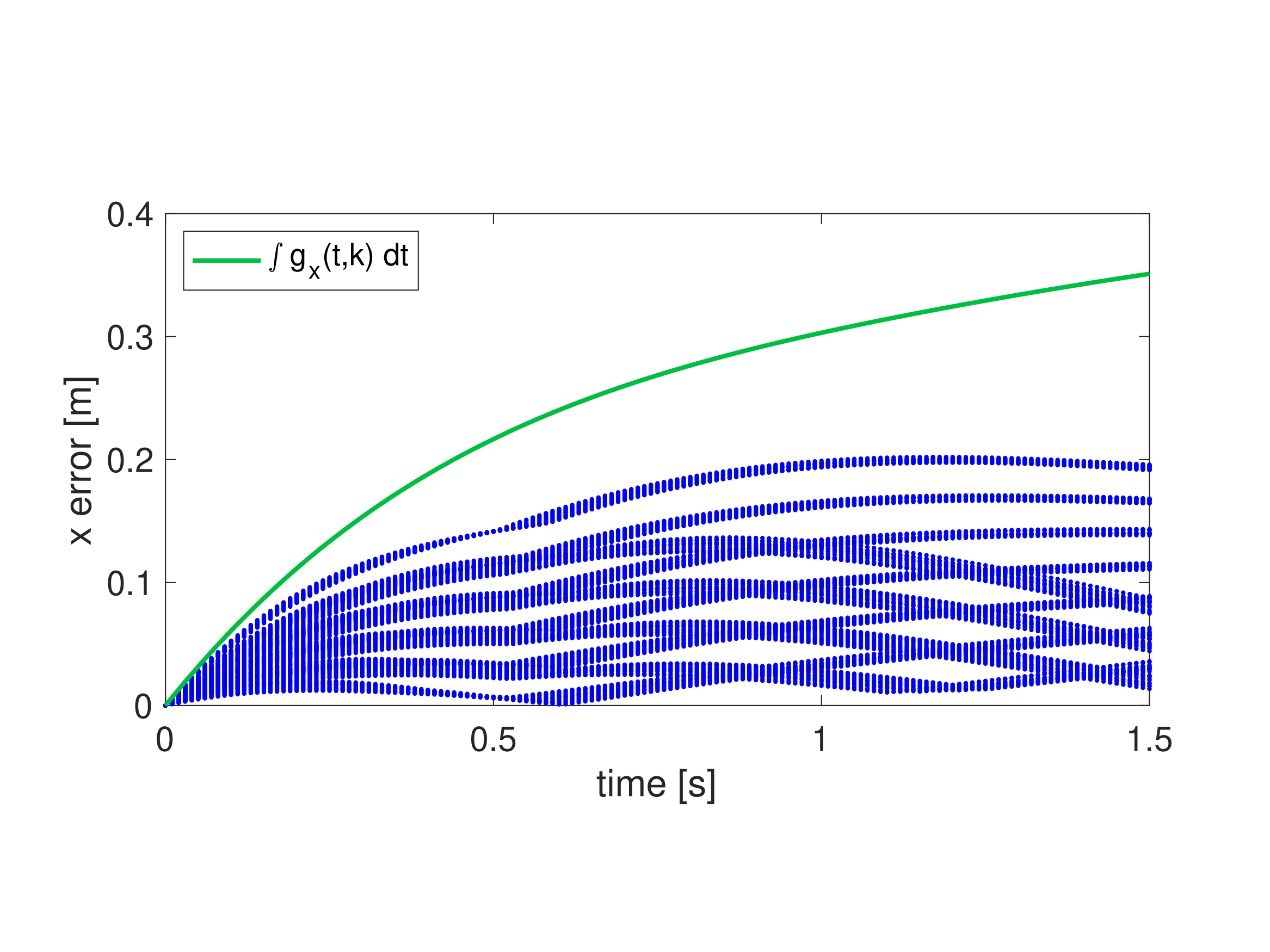
Assumption[8, Asm. 7]: for each shared coordinate \(i\in\{1,\dots,n_Z\}\) there exists a bounded, Lipschitz \(g_i:[0,T]\times Z\times K\to\mathbb R\) that conservatively bounds the cumulative tracking error between the high-fidelity \(\bar z_i\) and trajectory-producing \(z_i\): \[
\max_{\bar z\in A_z}\;\bigl|\bar z_i(t;\bar z_0,k)-z_i(t;z_0,k)\bigr|\;\le\;\int_0^t g_i(\tau,z,k)\,d\tau,
\]\(\forall\,z\in Z,\,t\in[0,T],\,k\in K\).
Why “worst-case”:\(g_i\) is the upper envelope over the family of sampled error trajectories — it must dominate the largest observed error at every \(t\). Only the worst realisation drives FRS conservatism.
Rover lateral-error fit at v0 = 1.94 m/s, ω0 = 0.95 rad/s (Kousik et al. 2020, Fig. 3a). Blue dashed: sampled tracking-error trajectories under the PD controller. Green solid: polynomial gx(t) that conservatively envelopes all of them — the worst-case envelope baked into Standard RTD's FRS.
Step 1 — Absorb \(g\) into the dynamics. Define the trajectory-tracking model with worst-case disturbance signal \(d\in L_d:=L^1([0,T],[-1,1]^{n_Z})\)[8, eq. (13)]: \[
\dot{\tilde z}(t)\;=\;f(t,\tilde z(t),k)\;+\;g(t,\tilde z(t),k)\circ d(t).
\]
Step 2 — FRS definition[8, eq. (18), § III.A]. The set of \(xy\)-subspace positions reachable by a robot described by the high-fidelity model while tracking parameterised trajectories from the trajectory-producing model, despite tracking error, over the horizon \(T\): \[
\begin{aligned}
\mathcal X_{\mathrm{FRS}}\;=\;\Bigl\{(x,k)\in X\!\times\! K\;\big|\;
&\exists\,z_0\in Z_0,\;\tau\in[0,T],\;d\in L_d\;\text{ s.t. }\;x=\mathrm{proj}_X\!\bigl(\tilde z(\tau)\bigr),\\
&\text{where }\;\dot{\tilde z}(t)=f(t,\tilde z(t),k)+g(t,\tilde z(t),k)\circ d(t)\\
&\text{a.e. }t\in[0,T],\;\tilde z(0)=z_0\Bigr\}.
\end{aligned}
\] Each fixed \(k\) slices a spatial tube
Obstacles are compact, connected, static subsets of \(X\); finite count \(n_{\mathrm{obs}}\) within sensor horizon at any instant [8, Def. 5]
Sensor horizon \(D_{\mathrm{sense}}\) is a radius around the robot within which size, shape, and location of every obstacle is known; occlusions and unexplored regions are treated as static obstacles [8, Asm. 5]
State-estimation buffer[8, Asm. 6]: every sensed obstacle is Minkowski-summed with \([-\varepsilon_x,\varepsilon_x]\!\times\![-\varepsilon_y,\varepsilon_y]\) before being passed to the planner
Geometric buffer + discretization[8]:\[
X_{\mathrm{obs}}^b=X_{\mathrm{obs}}\oplus\mathcal B(b),
\]\[
X_p=\texttt{discretizeObs}(X_{\mathrm{obs}}^b,r,a),
\] where \(b\) is a user-chosen buffer, \(r\) is the point spacing required so the robot’s footprint cannot fit between samples, \(a\) bounds arc-length around concave corners.
T2 Backup. RTD Core — Online Optimization OptK
OptK program[8, Prog. \((\mathrm{OptK})\)]: evaluate the offline polynomial \(w^l\) at each sensed obstacle point \(p\in X_p\): \[
\min_{k\in K}\;J(k)\quad\text{s.t.}\quad w^l(p,k)<1,\;\;\forall\,p\in X_p.
\]
Receding-horizon loop[8, Alg. 2]: at iteration \(j\), concurrently:
Apply\(u_{k_j^\star}\) to the robot for \([t_j,t_j+\tau_{\mathrm{plan}})\)
Sense → buffer → discretize → OptK → execute
T2 Backup. RTD Core — Parameter → Trajectory
In our turtlebot implementation, \(k=(k_1,k_2)\in[-1,1]^2\) are normalized, dimensionless knobs. The unit square is exactly the domain over which the offline FRS polynomial \(w^l(x,k)\) is fitted — no physical units enter until decode time.
Asymmetric \(k_2\) avoids spending half of \(K\)-space on reverse motion the planner doesn’t want
Step 2 — Dubins-unicycle two-phase trajectory:\[
\dot x=v(t)\cos\theta,\;\;\dot y=v(t)\sin\theta,\;\;\dot\theta=\omega(t),
\] with \(v(t)=v_{\mathrm{des}}\,s(t)\), \(\omega(t)=\omega_{\mathrm{des}}\,s(t)\), and braking scale: \[
s(t)=\begin{cases}1,&0\le t\le t_{\mathrm{plan}}\\[2pt]\max\!\bigl(0,\tfrac{t_{\mathrm{stop}}-(t-t_{\mathrm{plan}})}{t_{\mathrm{stop}}}\bigr),&t_{\mathrm{plan}}\le t\le T\end{cases}
\] where \(T=t_{\mathrm{plan}}+t_{\mathrm{stop}}\). Typical: \(t_{\mathrm{plan}}=0.5\) s, \(t_{\mathrm{stop}}=1.0\) s ⇒ one trajectory spans 1.5 s of horizon.
T2 Backup. RTD Core — Dubins Example: Planning vs High-Fidelity
The previous slide showed how \((k_1,k_2)\) decode to a Dubins-style trajectory. This is relevant, for example, in the case of a 5-D high-fidelity truth model versus a 2-D trajectory-producing (planning) model.
\((k_1,k_2)\)constant over \([0,T]\) — one parameter per planning iteration
Heading is implicit:\(\theta(t)=k_1 t\) (closed form) — no \(\theta\) state needed
\((x_{c,0},y_{c,0})\) = the high-fidelity centre-of-mass at the start of each iteration (planning frame anchor)
No saturation, no actuator dynamics — algebraically clean ⇒ tractable for offline SOS / FRS computation
Closing the gap — PD tracker[8, Ex. 3]. A simple PD controller \(u_k(t,\bar z)\) drives the 5-D \(\bar z\) to follow the 2-D Dubins reference: \[
u_k=\begin{bmatrix}\beta_\theta(k_1 t-\theta)+\beta_\omega(k_1-\omega)+\beta_y\,e_y\\\beta_v(k_2-v)+\beta_x\,e_x\end{bmatrix},\qquad
\begin{bmatrix}e_x\\e_y\end{bmatrix}=R(\theta)^\top\!\begin{bmatrix}x-x_c\\y-y_c\end{bmatrix}.
\] Whatever residual mismatch this PD leaves behind is exactly the tracking error that the worst-case envelope \(g(t)\) (slide 2) bounds — and the FRS (slide 3) over-approximates by union over \(d\in L_d\).
Every parameterised plan ends in a built-in brake. The FRS verifies the entire \(T=t_{\mathrm{plan}}+t_{\mathrm{stop}}\) window of every candidate \(k\), but the planner only commits the first \(t_{\mathrm{plan}}\) before re-planning. The braking tail is already certified safe by construction — no separate fail-safe controller is needed.
Why the stop is safe — three properties of \(s(t)\):
Terminal zero — \(s(T)=0\)exactly, so \(v\) and \(\omega\) are commanded to zero at the trajectory’s end.
Monotone decay — \(s\) is non-increasing on \([t_{\mathrm{plan}},T]\), so neither speed nor turn rate ever exceeds its planning-phase value during braking.
Pre-committed failsafe — the FRS already over-approximates the full \(T\)-window of every accepted \(k\), so the brake is part of the certificate, not an addition to it.
Failsafe trigger. If OptK returns no feasible \(k_{j+1}^\star\) in the next iteration, just keep executing \(k_j^\star\) — it brakes itself to rest inside the FRS-verified safe set.
T2 Backup. RTD-RAX — MMR: The Inclusion Function
For \(\dot x=f(x,u,w)\) with \(f\in C^1\), \(x\in\mathbb R^n\), \(u\in\mathbb R^m\), \(w\in\mathbb R^p\)[6]. Let \(\mathbb{IR}^n\) denote the set of intervals \([\underline a,\overline a]\subset\mathbb R^n\).
Inclusion function[6, eq. (2)]. A map \[
\mathsf F=[\underline{\mathsf F},\overline{\mathsf F}]:\mathbb{IR}^n\!\times\!\mathbb{IR}^m\!\times\!\mathbb{IR}^p\to\mathbb{IR}^n
\]includes\(f\) if for every\((x,u,w)\) in the input intervals, \[
f(x,u,w)\;\in\;\mathsf F\bigl([\underline x,\overline x],[\underline u,\overline u],[\underline w,\overline w]\bigr).
\]
Reads as:\(\mathsf F\) takes interval inputs and returns an interval output that contains every possible value of \(\dot x\) — no matter which point inside the input intervals was the truth.
Important: \(\mathsf F\) is a static set-valued bound. It is not yet a dynamical system — just a snapshot guarantee at one instant in time. The next slide turns this static bound into the embedding system \(\mathsf E\) that you can actually integrate.
Southeast order on \(\mathbb R^{2n}\): \((x,x')\preceq_{\mathrm{SE}}(y,y')\iff[y,y']\subseteq[x,x']\).
Given the inclusion function \(\mathsf F\) from the previous slide, we now construct the \(2n\)-dimensional embedding system\(\mathsf E\) — a single ODE whose state is the entire interval \((\underline x,\overline x)\).
Partial-replacement notation[6].\(x_{[i:y]}\in\mathbb R^n\) is the vector \(x\) with its \(i\)th component replaced by \(y_i\). So \(\overline x_{[i:\underline x]}\) = upper-bound vector with the \(i\)th coordinate “tightened” down to the lower bound.
When updating \(\dot{\underline x}_i\), the \(i\)th coordinate of the upper bound is collapsed to the lower bound (and symmetrically for \(\dot{\overline x}_i\)). Breaking \(\mathsf F\)’s symmetry this way is what turns the static bound into a dynamical\(2n\)-dim ODE whose flow is monotone in the southeast order — the property that earns “mixed monotone.”
\(\mathsf F\) vs \(\mathsf E\) side-by-side:
\(\mathsf F\) — inclusion function
\(\mathsf E\) — embedding system
Type
static, set-valued
dynamical, \(2n\)-dim ODE
Inputs
interval \((\underline x,\overline x,\dots)\)
same
Output
interval bound on \(\dot x\)
rate \((\dot{\underline x},\dot{\overline x})\)
Built from
\(f\) + interval analysis
\(\mathsf F\) + partial replacement
Use
snapshot bound
integrate → tube
Inclusion functions bound\(f\) at one instant; embedding systems propagate that bound through time.
The embedding system \(\mathsf E\) inherits two structural properties from the partial-replacement construction. These are what make it useful, not just well-defined.
Property 1 — Monotonicity of the flow \(\Phi^{\mathsf E}\)[6, eq. (7)]. If \[
(\underline x_0,\overline x_0)\preceq_{\mathrm{SE}}(\underline x'_0,\overline x'_0),
\]\[
[\underline u,\overline u](t)\preceq_{\mathrm{SE}}[\underline u',\overline u'](t)\;\;\forall\,t\!\ge\!0,
\]\[
[\underline w,\overline w](t)\preceq_{\mathrm{SE}}[\underline w',\overline w'](t)\;\;\forall\,t\!\ge\!0,
\] then for every \(t\ge 0\), \[
\Phi^{\mathsf E}(t;\cdot)\preceq_{\mathrm{SE}}\Phi^{\mathsf E}(t;\cdot').
\]
Tighter interval inputs (initial state, control, disturbance) yield tighter interval outputs at every horizon. The embedding flow respects containment of boxes through time.
Property 2 — Reachable-tube guarantee[6, eq. (8)]. For any \(x_0\in[\underline x_0,\overline x_0]\) and admissible signals \(u(\cdot),w(\cdot)\), \[
\phi(T;x_0,u,w)\;\in\;[\![\Phi^{\mathsf E}(T;[\underline x_0,\overline x_0],[\underline u,\overline u],[\underline w,\overline w])]\!].
\]
The bracket-bracket \([\![\cdot]\!]\) casts the \(2n\)-dim embedding state back into an \(n\)-dim interval — that interval contains every possible true-state trajectory.
Integration of the \(2n\)-dim ODE \(\mathsf E\) produces a rigorous hyperrectangular over-approximation of the true reachable set
The embedding-system theory is agnostic to how you build \(\mathsf F\). Two recipes for bounding \(f\) over an interval input[6], in increasing tightness:
1. Natural inclusion — interval arithmetic on \(f\): \[
\underline{\mathsf F}_i,\;\overline{\mathsf F}_i\;\;\text{from interval-evaluating each operator in }f_i.
\]
Easy: drop-in for any \(f\) written in elementary operators (\(+,-,\times,\sin,\exp,\dots\)).
Loose: suffers from the dependency problem — if \(x_1\) appears twice in \(f\) (e.g. \(x_1^2\)), each occurrence is bounded independently. The output box bloats even though both occurrences are the same variable.
2. Mixed-Jacobian inclusion[6, eq. (13)]. Bound \(f(x,u,w)-f(x',u',w')\) by a matrix set\(\mathcal M\,(x-x')\) derived from \(\partial f/\partial x\) on the box: \[
f(x,\cdot)-f(x',\cdot)\;\in\;\mathrm{co}\bigl\{\partial_x f([\underline x,\overline x])\bigr\}\,(x-x').
\]
Tighter than natural — the dependency problem is eliminated for terms whose Jacobian has sign-stable patterns over the box.
Computed via interval matrices on \(\partial_x f\); supported by mjacM in immrax.
Trade-off. Mixed-Jacobian needs interval matrix products at every integration step — pricier than natural’s interval arithmetic. Pick the loosest recipe that still gives the conservatism budget the application needs.
Problem: MMR integration gives interval bounds \([\underline x(t_k),\overline x(t_k)]\) at discrete times \(t_k = k\Delta t\). A naive check at \(\{t_k\}\) can miss collisions that happen between samples. Solution used by RTD-RAX [9]: construct the swept interval hull over \([t_k, t_{k+1}]\) from a one-sided bound on \(\dot{\underline x}, \dot{\overline x}\): \[
\mathrm{Hull}_k \;=\; \bigl[\,\min\{\underline x(t_k), \underline x(t_{k+1})\} - \rho\Delta t,\;\; \max\{\overline x(t_k), \overline x(t_{k+1})\} + \rho\Delta t\,\bigr]
\] with \(\rho\) an a priori Lipschitz constant of the embedding RHS (certified by the same immrax framework).
Certification guarantee: reachable set on \([t_k, t_{k+1}]\) is contained in \(\mathrm{Hull}_k\) (proof by continuity + Lipschitz bound)
Cost: constant per step (one max/min + one vector add)
Conservatism:\(O(\Delta t)\) — tightens with smaller time step; step chosen to keep total FRS-inflation comparable to Standard RTD
Without swept hulls, RTD-RAX would need an expensive inter-sample check (e.g., interval Taylor, verified ODE integration) at every \(k\) — killing real-time performance. The hull trick is the engineering step that makes the online MMR certificate tractable inside the 100 ms planning budget.
T2 Backup. RTD-RAX — Repair
Given a rejected candidate \(k^\star\) (with collision index \(j^\star\) from the MMR online check) [9]:
Speed back-off:\(k_2 \leftarrow \zeta_v\, k_2^\star\) with \(\zeta_v\in(0,1)\) → shorter trajectory time, tube grows less under uncertainty
Lateral push: shift \(k_1\) orthogonal to the obstacle normal at the counter-example; reuse the same neighbourhood of the rejected \(k^\star\)
Buffer tightening: inflate the obstacle buffer \(\delta_{j^\star}\) locally and re-solve the NLP over the non-inflated FRS
Verify each repair candidate by re-integrating the MMR embedding under the measured disturbance bound \([\underline w,\overline w]\); execute the first candidate whose tube stays collision-free over \([t,t+T]\)
Fail-safe: if no repair candidate certifies within the 100 ms planning budget, the previously executed plan’s fail-safe braking segment is committed (guaranteed safe by construction of the RTD family). Cost per cycle (Case 3, seed 32): mean \(10.5\) ms (matches Std RTD); p95 \(37.4\) ms (vs. \(21.9\) Std) — growth is entirely in the tail when repair fires [9].
T2 Backup. RTD-RAX — Full Icy Corridor
Full “icy corridor” benchmark [9]: multi-gap course with randomised disturbance patches and road-edge obstacles. RTD-RAX completes the course; Standard RTD aborts or collides across seeds.
50-seed randomised course with mixed obstacle + disturbance scenarios [9]
Full preliminary-work website: github.com/evannsm/rtd-rax
T2 Backup. RL-STL — Robustness & Plan
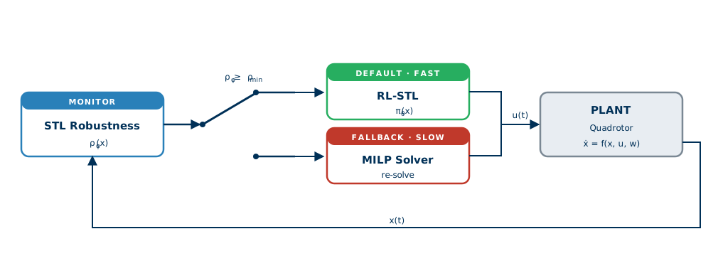
Core Idea: run policy \(\pi_\theta\) (2 ms) instead of MILP (tens of ms). Only re-solve MILP when \(\rho^\varphi\) drops below threshold
RL-STL Plan:
Offline: Train RL policy to imitate what the a particular STL policy’s MILP would return
At Runtime:
STL Monitor: compute I-STL robustness at each iteration
Use RL-STL policy by default
Trigger Condition: if robustness falls below minimum value → solve traditional MILP until robustness is adequate
STL robustness\(\rho^\varphi(\mathbf x, t)\) quantifies how much margin a trajectory \(\mathbf x\) has to satisfying \(\varphi\) at time \(t\)[4]:
T3 Backup. Switching & Inoculation
Thrust III · Backup Details
T3 Backup. Inoculation — Synthesis
Proposed Thrust 3 synthesis — extends the preliminary I-STL RTA[4]to post-fault recovery under cyber threat[14].
Under fault class \(\mathcal F_j\) identified (by NSF collaborator) via STL specification \(\varphi_j\):
Viability kernel\(\mathcal V_j = \{x_0 : \exists u(\cdot),\;x(t)\in\mathcal X_{\mathrm{safe}}\;\forall t\geq 0\}\) for post-fault dynamics is generally intractable online
Construct parameterized backup controller \(u_{b,j}\) whose certified operating domain \(\mathcal S_j \subseteq \mathcal V_j\) is forward-invariant under post-fault dynamics
Certification: propagate MMR tube [7, 15] under \(u_{b,j}\) starting from \(\mathcal S_j\); if \([\underline x(t),\overline x(t)]\subseteq\mathcal X_{\mathrm{safe}}\) for \(t\in[0,T_{\mathrm{rec}}]\), add \((u_{b,j}, \mathcal S_j, \varphi_j)\) to library
Online matching: locality-sensitive hashing of fault signatures → constant-time lookup of matching \(u_{b,j}\); fallback to RTA tube during search
Contract with NSF collaborators: they deliver \((\hat{\mathcal F}_j, \hat\varphi_j)\); we deliver the certified pair \((u_{b,j}, \mathcal S_j)\)
M. E. Cao, A. Harapanahalli, E. Morales-Cuadrado and S. Coogan, “Trajectory tracking for systems with unknown time-varying disturbances,”IEEE OJ-CSYS (submitted), 2026.